Why I Wanted To Look Inside A Model
Most of my previous AI projects focused on making a model do something. I taught a small base model to emit reasoning traces, trained models with RL, and even pre-trained a language model from random weights. In each project, I mostly understood the model by looking at what went in and what came out.
This time, I wanted to try something different: look inside a model, identify a feature that represented something understandable, and directly push the model toward that feature during generation.
I wanted to take a small open model, build the complete pipeline myself, find an interesting feature inside it, and test whether it was actually causal. The project was inspired by Anthropic's Golden Gate Claude experiment, in which researchers found a feature related to the Golden Gate Bridge and artificially activated it until Claude mentioned the bridge in unrelated answers. I wanted to try a smaller version of that idea on Qwen3-4B-Base.
What A Sparse Autoencoder Does
A transformer's residual stream is a large vector that carries information through the model. A single direction within that vector does not always represent one concept cleanly because models can pack many overlapping concepts into the same activation space.
A sparse autoencoder, or SAE, tries to unpack that space into a much larger set of sparse features. Its encoder turns a residual activation into feature activations, most of which are forced to stay inactive for any given token. Its decoder then tries to reconstruct the original residual activation from the smaller set of active features.
One feature might activate on years in citations, another on legal disclaimers, and another on cooking instructions. Once I had those directions, I could do more than observe them: I could add one back into the model's residual stream during generation and see whether the output changed as predicted.
The Setup
I used Qwen3-4B-Base and hooked into the residual stream at layer 20. Qwen3-4B has 36 layers, and the residual stream at this layer has a width of 2560.
I used FineWeb-Edu as the text source. I tokenized 50M tokens, ran them through Qwen, and cached the layer 20 activations. Caching meant I did not have to repeatedly load and run the base model while training different SAEs.
The main SAE expanded each 2560-dimensional activation into 10240 possible features.
model_name: /vol/models/Qwen3-4B-Base
hook_name: model.layers.20
d_in: 2560

architecture: standard
expansion_factor: 4
d_sae: 10240

training_tokens: 52428800
l1_coefficient: 5.0
I ran the pipeline on Modal and used SAELens for the SAE training. The whole project was config-driven. I had separate configs for tokenization, activation caching, training, feature dashboards, autointerp, and steering. This made it much easier to run small smoke tests before spending money on the larger jobs.
Finding A Useful Sparsity Level
The most important training choice was the L1 coefficient, which controls how strongly the SAE is penalized for activating too many features. If the value is too low, the SAE reconstructs activations well but uses too many features at once, which makes the features harder to interpret. If the value is too high, the features become sparse but many of them die and never activate.
I compared runs with L1 values of 1, 2, and 5. The L1 5 run reached an average L0 of roughly 55, meaning around 55 features were active per token on average. That result was much closer to the sparse representation I wanted, but it also produced many dead features.
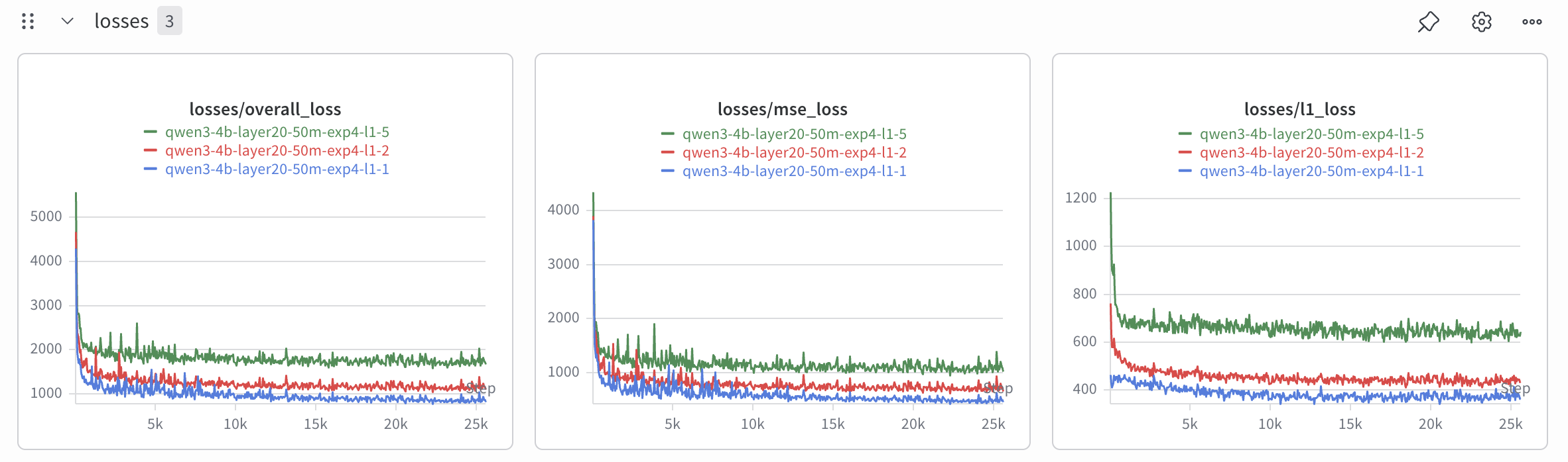
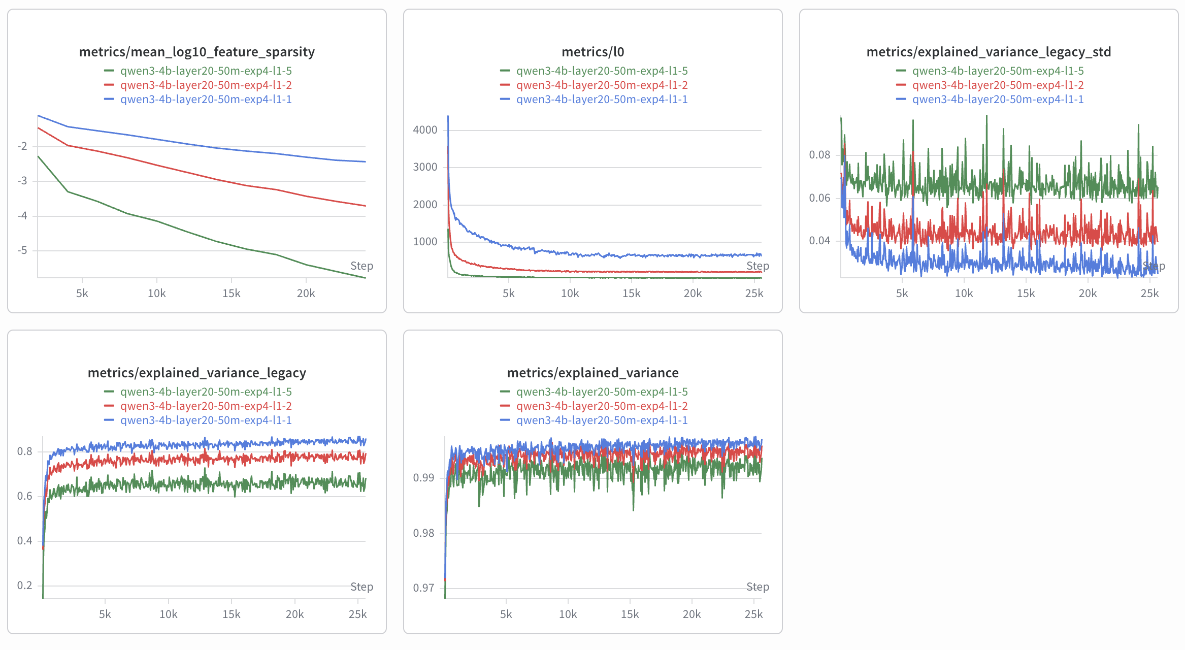
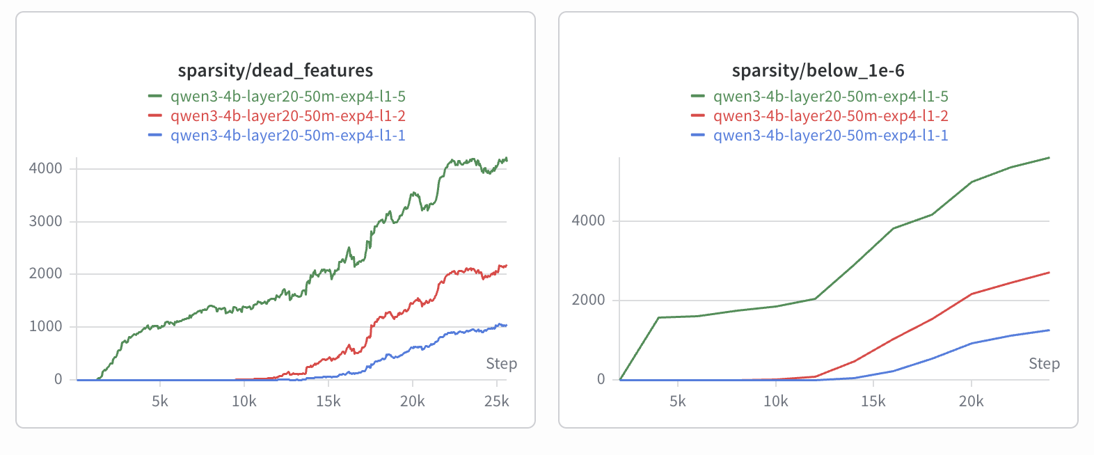
This result taught me my first major lesson from the project: better reconstruction does not automatically produce a better SAE for interpretability. The L1 1 run reconstructed more cleanly, but the L1 5 run gave me a much more useful sparse feature space. If I repeat this project, I would like to try a TopK SAE, where the number of active features is controlled directly instead of through an L1 penalty.
Labeling Thousands Of Features
After training, I built a feature dashboard that stored the highest-activating token windows for each feature. Reviewing thousands of examples manually would have taken far too long, so I used LLM autointerp.
For every feature, I gave an LLM its top activating examples and asked it to return a short label, confidence score, and reason.
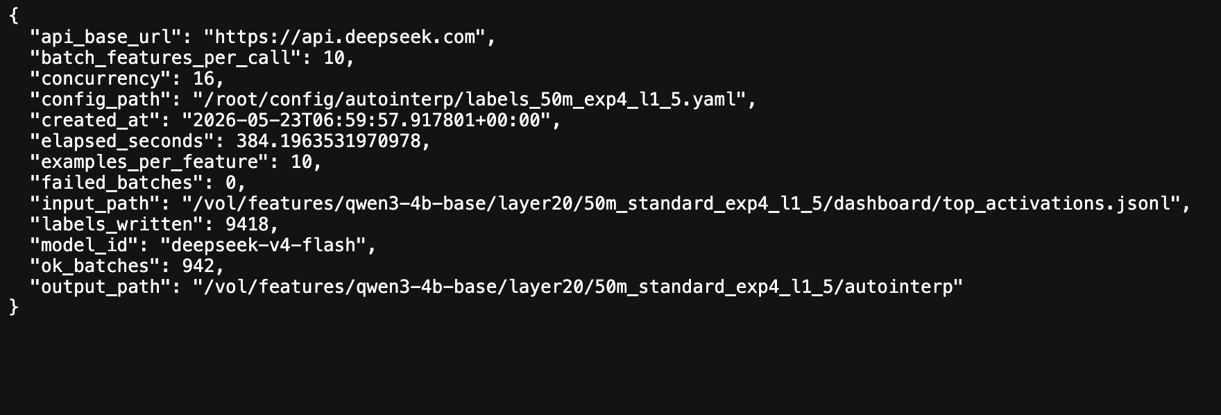
I used the deepseek-v4-flash non-thinking model because it was cheap and strong enough for this repetitive labeling task. I batched 10 features per API request, used 10 examples per feature, and ran the requests with concurrency 16 inside a Modal CPU function.
model_id: deepseek-v4-flash
batch_features_per_call: 10
examples_per_feature: 10
concurrency: 16
temperature: 0.0
The full run labeled 9418 features in about 384 seconds without any failed batches.
Some labels were boring token or formatting features, which is expected. I found features for years in citations, repeated dots in tables, institution headers, and spaces before numbers.
But there were also more semantic features:
- feature
703: exercise and physical activity
- feature
3311: cooking instructions
- feature
7771: biblical moral language
- feature
665: alternative medicine and wellness
- feature
9142: military attacks and offensives
Steering The Cooking Instructions Feature
I picked feature 3311, labeled cooking instructions, because I could easily test it with neutral prompts.
The steering method was simple. I took the decoder direction for feature 3311, normalized it, multiplied it by a steering strength called alpha, and added it to the layer 20 residual stream during generation.
direction = W_dec[feature_id]
direction = direction / direction.norm()

hidden = hidden.clone()
hidden[:, -1, :] = hidden[:, -1, :] + alpha * direction
I tested alpha values from -60 to 80 using the same neutral prompts.
The clearest example began with this prompt:
Write a short paragraph about a simple daily routine.
With no steering, Qwen wrote a normal paragraph about waking up, eating breakfast, exercising, working, and relaxing.
At alpha 40, the same prompt became:
A simple daily routine can be made by adding a few drops of water
to a cup of warm water and stir it. Add a teaspoon of honey and
stir again. Add a teaspoon of lemon juice and stir again...
The prompt never asked for a recipe, yet the model started producing ingredients and procedural cooking language. At alpha 60 and 80, the cooking direction became stronger, but the output collapsed into repetition:
Add a little water and stir. add a little water and stir.
add a little water and stir...
This was the most useful result for me. Adding its decoder direction causally pushed generation toward cooking instructions. But the experiment also showed how fragile naive steering is. More steering did not mean a better result. Past a certain point, the intervention damaged the model's ability to generate coherent text.
What Happened In The Negative Direction
Negative alpha values often shifted the output toward mathematical, formal, or academic text. For one prompt, alpha -60 produced a completion about the Tower of Hanoi. Other outputs discussed contest problems and algebraic geometry.
This result was interesting because both directions produced coherent shifts. Positive values pushed toward cooking and procedural language, while negative values often moved toward formal academic content. I would not call this proof that mathematics is the exact opposite of cooking inside Qwen. A negative decoder direction can move the model outside the normal activation distribution, and steering results can depend heavily on the layer, prompt, position mode, and alpha.
The 500GB Problem
The Modal volume eventually grew past 500GB because it contained the model weights, tokenized datasets, cached activations, multiple SAE runs, dashboards, labels, and steering outputs.
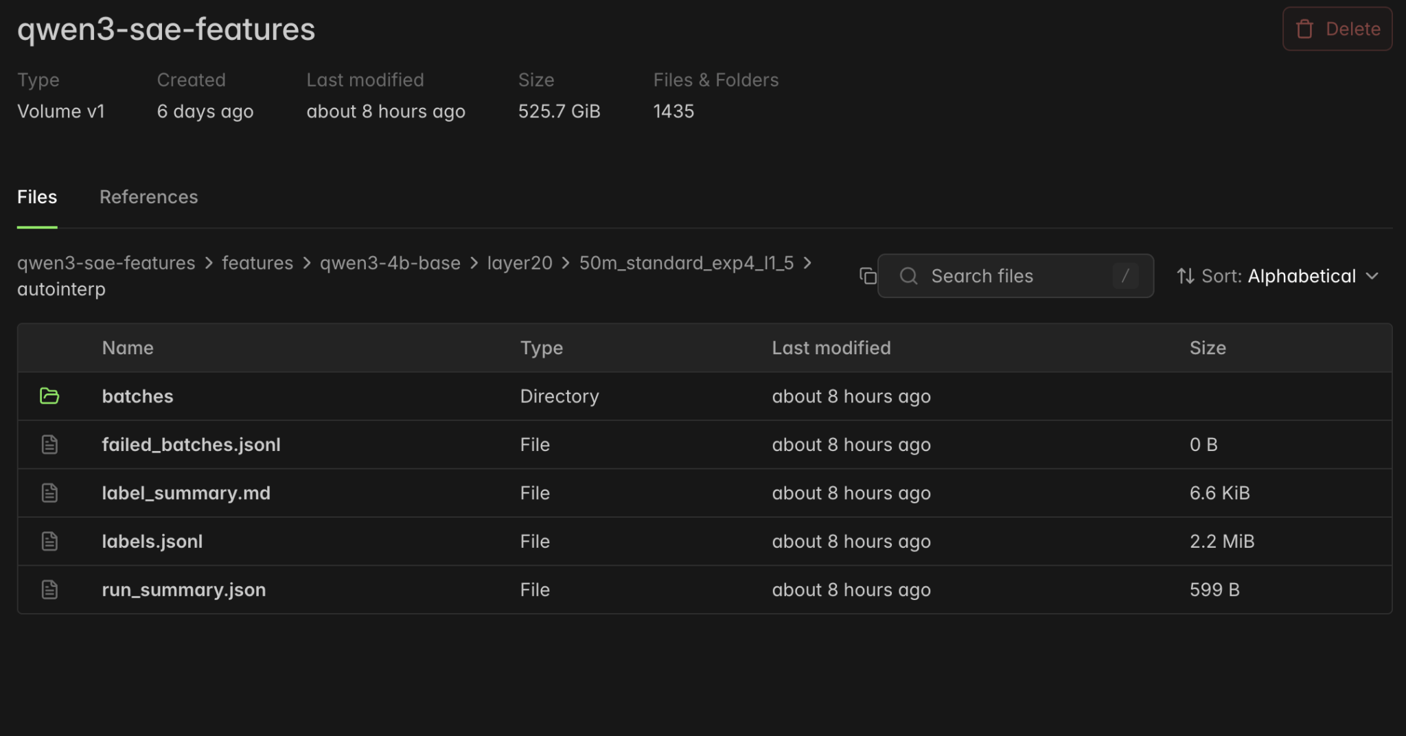
I eventually deleted the volume because keeping more than 500GB of experimental artifacts around was not worth it. Before deleting it, I saved the important JSONL labels, summaries, configs, and steering results locally. This experience taught me another practical lesson: mechanistic interpretability experiments are not only compute-intensive; activation caching can also become a storage problem very quickly.
What I Learned
Before this project, looking inside a model sounded much more mysterious to me than training one. Now I have a rough mental model of the complete loop: choose an activation space, cache activations, train an SAE, inspect the top-activating examples, use autointerp to find candidate features, and intervene during generation to test whether a feature is causal.
I found a learned direction inside Qwen3-4B-Base that was associated with cooking instructions. I turned that direction up and watched neutral text become recipe-like. Then I turned it up too far and watched the model collapse into repetitive stirring.
Links
Project
Model And Data
Why I Wanted To Look Inside A Model
Most of my previous AI projects focused on making a model do something. I taught a small base model to emit reasoning traces, trained models with RL, and even pre-trained a language model from random weights. In each project, I mostly understood the model by looking at what went in and what came out.
This time, I wanted to try something different: look inside a model, identify a feature that represented something understandable, and directly push the model toward that feature during generation.
I wanted to take a small open model, build the complete pipeline myself, find an interesting feature inside it, and test whether it was actually causal. The project was inspired by Anthropic's Golden Gate Claude experiment, in which researchers found a feature related to the Golden Gate Bridge and artificially activated it until Claude mentioned the bridge in unrelated answers. I wanted to try a smaller version of that idea on Qwen3-4B-Base.
What A Sparse Autoencoder Does
A transformer's residual stream is a large vector that carries information through the model. A single direction within that vector does not always represent one concept cleanly because models can pack many overlapping concepts into the same activation space.
A sparse autoencoder, or SAE, tries to unpack that space into a much larger set of sparse features. Its encoder turns a residual activation into feature activations, most of which are forced to stay inactive for any given token. Its decoder then tries to reconstruct the original residual activation from the smaller set of active features.
One feature might activate on years in citations, another on legal disclaimers, and another on cooking instructions. Once I had those directions, I could do more than observe them: I could add one back into the model's residual stream during generation and see whether the output changed as predicted.
The Setup
I used Qwen3-4B-Base and hooked into the residual stream at layer
20. Qwen3-4B has36layers, and the residual stream at this layer has a width of2560.I used FineWeb-Edu as the text source. I tokenized
50Mtokens, ran them through Qwen, and cached the layer20activations. Caching meant I did not have to repeatedly load and run the base model while training different SAEs.The main SAE expanded each
2560-dimensional activation into10240possible features.I ran the pipeline on Modal and used SAELens for the SAE training. The whole project was config-driven. I had separate configs for tokenization, activation caching, training, feature dashboards, autointerp, and steering. This made it much easier to run small smoke tests before spending money on the larger jobs.
Finding A Useful Sparsity Level
The most important training choice was the L1 coefficient, which controls how strongly the SAE is penalized for activating too many features. If the value is too low, the SAE reconstructs activations well but uses too many features at once, which makes the features harder to interpret. If the value is too high, the features become sparse but many of them die and never activate.
I compared runs with L1 values of
1,2, and5. The L15run reached an average L0 of roughly55, meaning around 55 features were active per token on average. That result was much closer to the sparse representation I wanted, but it also produced many dead features.This result taught me my first major lesson from the project: better reconstruction does not automatically produce a better SAE for interpretability. The L1
1run reconstructed more cleanly, but the L15run gave me a much more useful sparse feature space. If I repeat this project, I would like to try a TopK SAE, where the number of active features is controlled directly instead of through an L1 penalty.Labeling Thousands Of Features
After training, I built a feature dashboard that stored the highest-activating token windows for each feature. Reviewing thousands of examples manually would have taken far too long, so I used LLM autointerp.
For every feature, I gave an LLM its top activating examples and asked it to return a short label, confidence score, and reason.
I used the
deepseek-v4-flashnon-thinking model because it was cheap and strong enough for this repetitive labeling task. I batched10features per API request, used10examples per feature, and ran the requests with concurrency16inside a Modal CPU function.The full run labeled
9418features in about384seconds without any failed batches.Some labels were boring token or formatting features, which is expected. I found features for years in citations, repeated dots in tables, institution headers, and spaces before numbers.
But there were also more semantic features:
703: exercise and physical activity3311: cooking instructions7771: biblical moral language665: alternative medicine and wellness9142: military attacks and offensivesSteering The Cooking Instructions Feature
I picked feature
3311, labeledcooking instructions, because I could easily test it with neutral prompts.The steering method was simple. I took the decoder direction for feature
3311, normalized it, multiplied it by a steering strength called alpha, and added it to the layer20residual stream during generation.I tested alpha values from
-60to80using the same neutral prompts.The clearest example began with this prompt:
With no steering, Qwen wrote a normal paragraph about waking up, eating breakfast, exercising, working, and relaxing.
At alpha
40, the same prompt became:The prompt never asked for a recipe, yet the model started producing ingredients and procedural cooking language. At alpha
60and80, the cooking direction became stronger, but the output collapsed into repetition:This was the most useful result for me. Adding its decoder direction causally pushed generation toward cooking instructions. But the experiment also showed how fragile naive steering is. More steering did not mean a better result. Past a certain point, the intervention damaged the model's ability to generate coherent text.
What Happened In The Negative Direction
Negative alpha values often shifted the output toward mathematical, formal, or academic text. For one prompt, alpha
-60produced a completion about the Tower of Hanoi. Other outputs discussed contest problems and algebraic geometry.This result was interesting because both directions produced coherent shifts. Positive values pushed toward cooking and procedural language, while negative values often moved toward formal academic content. I would not call this proof that mathematics is the exact opposite of cooking inside Qwen. A negative decoder direction can move the model outside the normal activation distribution, and steering results can depend heavily on the layer, prompt, position mode, and alpha.
The 500GB Problem
The Modal volume eventually grew past
500GBbecause it contained the model weights, tokenized datasets, cached activations, multiple SAE runs, dashboards, labels, and steering outputs.I eventually deleted the volume because keeping more than
500GBof experimental artifacts around was not worth it. Before deleting it, I saved the important JSONL labels, summaries, configs, and steering results locally. This experience taught me another practical lesson: mechanistic interpretability experiments are not only compute-intensive; activation caching can also become a storage problem very quickly.What I Learned
Before this project, looking inside a model sounded much more mysterious to me than training one. Now I have a rough mental model of the complete loop: choose an activation space, cache activations, train an SAE, inspect the top-activating examples, use autointerp to find candidate features, and intervene during generation to test whether a feature is causal.
I found a learned direction inside Qwen3-4B-Base that was associated with cooking instructions. I turned that direction up and watched neutral text become recipe-like. Then I turned it up too far and watched the model collapse into repetitive stirring.
Links
Project
Model And Data
Tools And Reading